SAC

Topics: Reinforcement Learning

Introduction

Soft Actor-Critic (SAC) is a model-free, actor-critic, off-policy, RL algorithm that trains a stochastic policy following the Entropy Maximization framework in an Entropy-Regularized Reinforcement Learning environment. It is targeted at environments with continuous action spaces.

Objective

Standard RL agents maximize the expected return, whereas the goal of the SAC agent is to maximize both the expected return and the policy entropy. In other words, the agent aims to succeed at the task while acting as randomly as possible.

In a finite horizon setting, the objective function, augmented by the entropy term is as follows (1):
$J(\pi) = \sum_{t=0}^{T} \underset{(s_{t},a_{t}) \sim \rho_{\pi}}{\mathbb{E}} \biggr[ r(s_{t}, a_{t}) + \alpha \, \mathcal{H} \Bigr( \pi ( \cdot \vert s_{t}) \Bigr) \biggr]$
where $\alpha$ is the temperature parameter, also known as the entropy regularization coefficient.

In an infinite horizon setting, the objective becomes (1):
$J(\pi) = \sum_{t=0}^{\infty} \underset{(s_{t}, a_{t}) \sim \rho_{\pi}}{\mathbb{E}} \Biggr[ \sum_{l=t}^{\infty} \gamma^{l-t} \; \underset{ \substack{ s_{l} \sim p \\ a_{l} \sim \pi } }{\mathbb{E}} \biggr[ r(s_{t}, a_{t} ) + \alpha \, \mathcal{H} \Bigr( \pi ( \cdot \vert s_{t}) \Bigr) \Bigr \vert s_{t}, a_{t} \biggr] \Biggr]$
where $\gamma$ is the discount factor.

Temperature Parameter

The temperature parameter $\alpha$ is used to adjust the effect of the entropy term with respect to the environment reward in the return equation. It is a hyperparameter which needs to be carefully tuned, as it can degrade the performance of SAC significantly. It controls the level of exploration vs. exploitation.

If the temperature parameter is too high, then the entropy term will dominate the return and the policy will progress towards a highly stochastic policy, almost uniform. This means that the agent explores most of the time and does not exploit enough. On the other hand, if the temperature parameter is too small, the reward will dominate the return and the policy will progress towards a more deterministic policy. This means that the agent exploits most of the time and does not explore enough, which can lead to convergence to local optima.

There are 2 approaches when it comes to the temperature parameter $\alpha$ in SAC (3): one that uses a fixed temperature parameter (1), which needs to be tuned, and another that includes a constrained formulation that automatically tunes the temperature hyperparameter (2). A fixed $\alpha$ results in a simpler algorithm but requires tuning, whereas the second approach is more complex and is generally preferred by practitioners (3).

Algorithm Details

The derivation of the algorithm starts from the soft policy iteration algorithm, which is the general form for learning optimal maximum entropy policies that alternates between policy evaluation and policy improvement in the maximum entropy framework. It works for discrete action spaces

In policy evaluation, the soft Q-value is computed iteratively by applying the following Bellman backup operator $\tau^{\pi}$ (1):
$\tau^{\pi} Q(s_{t}, a_{t}) \triangleq r(s_{t}, a_{t}) + \gamma \, \underset{s_{t+1} \sim p}{\mathbb{E}} \Bigr[ V(s_{t+1}) \Bigr]$
where
$V(s_{t}) = \underset{a_t \sim \pi}{\mathbb{E}} \Bigr[ Q(s_{t}, a_{t}) − \alpha \, \text{log} \, \pi({a_t}\vert s_{t}) \Bigr]$
In the policy improvement step, the policy is updated towards the exponential of the new Q-function, which can guarantee that the new policy is an improvement over the previous one. In more detail, the Kullback-Leibler divergence is used to project the new policy into a constraint set. I NEED TO GO INTO THIS IN MORE DETAIL!
$\pi_{new} = \text{arg } \underset{\pi' \in \Pi}{\text{min }} \text{D}_{\text{KL}} \Biggr( \pi' (\cdot \vert s_{t}) \; \Biggr \| \frac{\text{exp}\Bigr(Q^{\pi_{old}}(s_t, \cdot) \Bigr) }{Z^{\pi_{old}} (s_t)} \Biggr)$
The SAC algorithm is for continuous action spaces, so the above soft policy iteration algorithm is approximated using neural networks. There are 2 main variations of the SAC algorithm: one that uses a value network (1) and one that does not (2). They both start from the same equations above. The first version keeps the value function in the equations whereas the second one replaces the value function with an expression of Q-function, and hence eliminates the need for a value network.

SAC with Value Network

The version of SAC with value network requires the following neural networks:

• value network: $V_{\psi}(s)$
• target value network: $V_{\bar{\psi}}(s)$
• 2 critic networks: $Q_{\theta_{1}}(s, a)$ and $Q_{\theta_{2}}(s, a)$
• actor network: $\pi_{\phi}(s)$

The updates of the networks follow directly from the equations of the soft policy iteration algorithm.

The **soft value network is trained to minimize the squared residual error (1):
$J_{V}(\psi) = \underset{s_{t} \sim D}{\mathbb{E}} \Biggr[ \frac{1}{2} \biggr( V_{\psi}(s_t) - \underset{a_t \sim \pi_{\phi}}{\mathbb{E}} \Bigr[ Q_{\theta}(s_t, a_t) - \alpha \, \text{log} \; \pi_{\phi}(a_t \vert s_t) \Bigr] \biggr) ^2 \Biggr]$
where $D$ is the replay buffer. Also, the minimum Q-value from the 2 critic networks is taken, a technique similar to double Q-learning and TD3.
The target value network can be updated using polyak averaging or periodic hard updates.

The soft Q-function networks can be trained to minimize the soft Bellman residual (1):
$J_Q(\theta) = \underset{(s_t, a_t) \sim D}{\mathbb{E}} \biggr[ \frac{1}{2} \Bigr( Q_{\theta}(s_t, a_t) - \hat{Q}_{\theta}(s_t, a_t) \Bigr) ^2 \biggr]$
with
$\hat{Q}_{\theta}(s_t, a_t) = r(s_t, a_t) + \gamma \, \underset{s_{t+1} \sim p}{\mathbb{E}} \Bigr[ V_{\bar{\psi}}(s_{t+1}) \Bigr]$
Finally, the actor network update relies on the reparameterization trick and has the following objective (1):
I NEED TO RESEARCH THE REPARAMETERIZATION TRICK!
$J_{\pi}(\phi) = \underset{\substack{s_t \sim D \\ \epsilon_t \sim \mathcal{N}}}{\mathbb{E}} \biggr[ \alpha \, \text{log } \pi_{\phi} \Bigr( f_{\phi}(\epsilon_t; s_t) \, \vert \, s_t \Bigr) - Q_{\theta} \Bigr(s_t, f_{\phi}(\epsilon_t; s_t) \Bigr) \biggr]$
Similarly to the value network update, the minimum of the Q-values from the critic networks is used in the actor network update.

SAC without Value Network

This version of SAC requires the following neural networks:

• 2 critic networks: $Q_{\theta_{1}}(s, a)$ and $Q_{\theta_{2}}(s, a)$
• 2 target critic networks: $Q_{\bar{\theta}_{1}}(s, a)$ and $Q_{\bar{\theta}_{2}}(s, a)$
• actor network: $\pi_{\phi}(s)$

The derivation starts from the same soft Q-function loss as above:
$J_Q(\theta) = \underset{(s_t, a_t) \sim D}{\mathbb{E}} \Biggr[ \frac{1}{2} \biggr( Q_{\theta}(s_t, a_t) - \Bigr( r(s_t, a_t) + \gamma \, \underset{s_{t+1} \sim p}{\mathbb{E}} \Bigr[ V_{\bar{\theta}}(s_{t+1}) \Bigr] \Bigr) \biggr) ^2 \Biggr]$
then replace the value equation by its definition (2):
$J_Q(\theta) = \underset{(s_t, a_t) \sim D}{\mathbb{E}} \Biggr[ \frac{1}{2} \biggr( Q_{\theta}(s_t, a_t) - \Bigr( r(s_t, a_t) + \gamma \, \underset{\substack{ s_{t+1} \sim p \\ a_{t+1} \sim \pi_{\phi}}}{\mathbb{E}} \Bigr[ Q_{\bar{\theta}}(s_{t+1}, a_{t+1}) − \alpha \, \text{log} \, \pi_{\phi}({a_{t+1}}\vert s_{t+1}) \Bigr] \Bigr) \biggr) ^2 \Biggr]$
The minimum of the target Q-values is used in the equation above.

The actor network is updated similarly to the first method.

Finally, the weights of the critic target networks are updates via polyak averaging or periodic hard updates.

Pseudocode

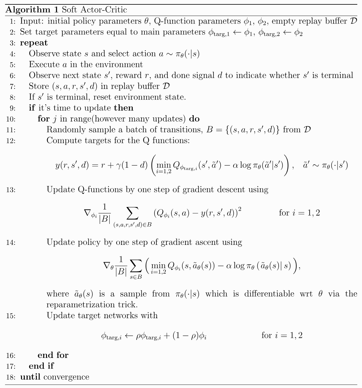
References

1. T. Haarnoja, A. Zhou, P. Abbeel, and S. Levine, “Soft Actor-Critic: Off-Policy Maximum Entropy Deep Reinforcement Learning with a Stochastic Actor,” Aug. 08, 2018, arXiv: arXiv:1801.01290. doi: 10.48550/arXiv.1801.01290.
2. T. Haarnoja et al., “Soft Actor-Critic Algorithms and Applications,” Jan. 29, 2019, arXiv: arXiv:1812.05905. doi: 10.48550/arXiv.1812.05905.
3. https://spinningup.openai.com/en/latest/algorithms/sac.html