Ornstein-Uhlenbeck Process

Topics: Stochastic Processes

Definition

The Ornstein-Uhlenbeck process is a stochastic process described though the stochastic differential equation (1):
$dx_t = -\theta(x_t - \mu) + \sigma \cdot dW_t$
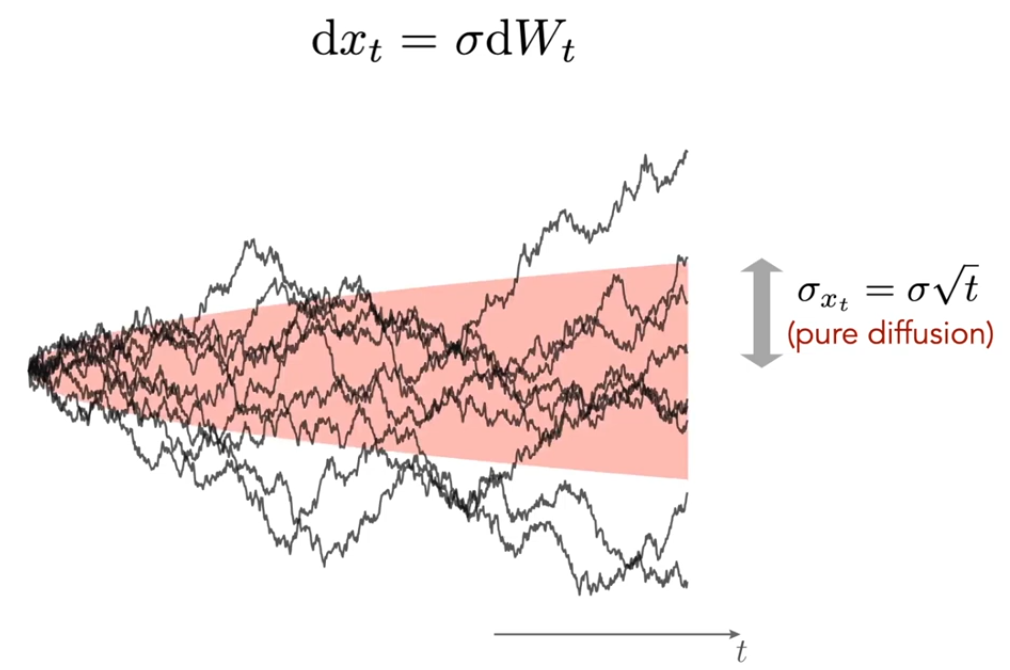
Stochasticity comes from the second term $\sigma \cdot dW_t$ where $W_t$ represents a Weiner process. If we have the second term alone $dx_t = \sigma \cdot dW_t$, then the process is pure diffusion; its standard deviation grows as square root of time, meaning that $x$ fluctuates without bounds: $\sigma_{x_t}=\sigma \sqrt{(t)}$ (1).

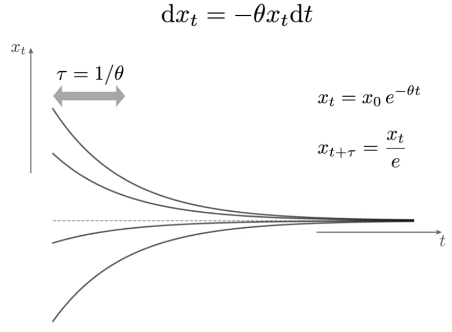
The first term is deterministic; it represents a restoring force that brings $x$ back to its mean value $\mu$. Without the second term, $dx_t = -\theta(x_t - \mu)$, $x$ would revert back to $\mu$ from any starting position exponentially in time with the relaxation rate set by $\theta$ (1).

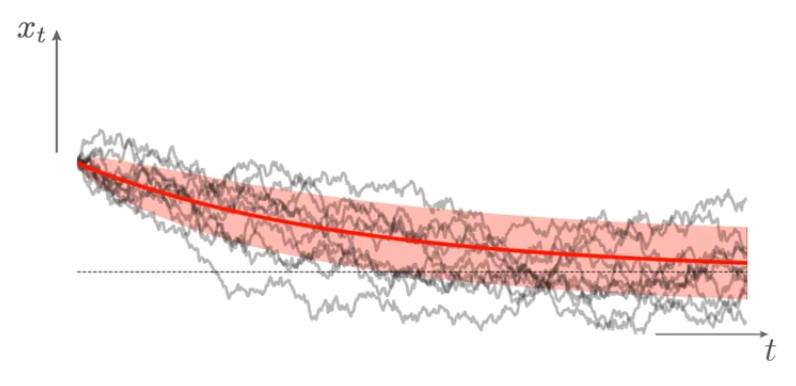
With both terms, we get the Ornstein-Uhlenbeck process: the second term drives the process by generating fluctuations, while the first term tries to suppress the fluctuations (1). The process is called mean-reverting because, over time, it tends to drift towards its mean value (2).

The further $x$ deviates from the mean, the larger the restoring effect becomes. In other words, the restoring term dominates near $\mu$, while the stochastic term dominates away from $\mu$ (1).

Statistical Properties

The Ornstein-Uhlenbeck is a stationary Gauss-Markov process, which means it is a Gaussian process, a Markov process, and is temporarily homogeneous (2).

The mean and variance of the process are:

$$\begin{align*} & mean = <x_{\Delta t} \vert x_0> = x_0 \, e^{-\theta \, \Delta t} + \mu \, (1 - e^{-\theta \, \Delta t}) \\ \\ & variance = Var( x_{\Delta t} \vert x_0 ) = \frac{\sigma ^2}{2 \theta} (1-e^{-2 \theta\, \Delta t}) \end{align*}$$

From the exponentials in the mean and variance equations, we can notice that the variance converges to its steady-state value twice as fast as the mean.

Simulation in Python

There are 2 ways to simulate the Ornstein-Uhlenbeck process in Python.

Analytical Solution

Given $x_0$ and $\Delta t$, we compute the mean and variance then sample $x_{\Delta t}$ from a Gaussian distribution (3).

$$\begin{align*} & First\; Iteration \\ \\ & mean(x_0) = <x_{\Delta t} \vert x_0> = x_0 e^{-\theta \Delta t} + \mu \left( 1-e^{-\theta \Delta t} \right) \\ \\ & Var(x_{\Delta t} \vert x_0) = \frac{\sigma ^2}{2 \theta} \left( 1-e^{-2 \theta \Delta t} \right) \\ \\ & x_{\Delta t} \sim \mathcal{N}(mean(x_0), Var) \\ \\ \\ \\ & Second\; Iteration \\ \\ & mean(x_{\Delta t}) = <x_{2 \Delta t} \vert x_{\Delta t}> = x_{\Delta t}\; e^{-\theta \Delta t} + \mu \left( 1-e^{-\theta \Delta t} \right) \\ \\ & Var(x_{2 \Delta t} \vert x_{\Delta t}) = \frac{\sigma ^2}{2 \theta} \left( 1-e^{-2 \theta \Delta t} \right) \\ \\ & x_{\Delta t} \sim \mathcal{N}(mean(x_{\Delta t}), Var) \\ \\ \\ \\ & N^{th}\; Iteration \\ \\ & x_{N \Delta t} \sim \mathcal{N}(mean(x_{(N-1)\Delta t}), Var) \\ \\ & N=\frac{T_{total}}{\Delta t} \end{align*}$$

Euler-Maruyama Solution

We can simulate the Ornstein-Uhlenbeck process using an alternative numerical integration method called Euler-Maruyama method. It is an approximate procedure to numercally solve stochastic differential equations (3).

$$\begin{align*} & dx_t = -\theta(x_t - \mu) + \sigma \cdot dW_t \\ \\ & x_{t+\Delta t} \approx x_t - \theta \; \Delta t \; (x_t - \mu) + \sigma \; \Delta W_t \\ \\ & where \;\; \sigma \; \Delta W_t \sim \mathcal{N}(0, \sigma^2 \Delta t) \\ \\ & <x_{t+\Delta t} \vert x_t> \approx x_t - \theta \, \Delta t \, (x_t - \mu) \\ \\ & Var(x_{t+\Delta t} \vert x_t) \approx \sigma^2 \, \Delta t \end{align*}$$

Autocorrelation

Autocorrelation is the degree of similarity of the stochastic variable at different times.

• with $\Delta t$ small with respect to $\tau$, there is high correlation
• as $\Delta t$ increases $(\Delta t > 0.5\tau)$, correlation decreases

Autocorrelation derivation (1):

$$\begin{align*} &<x_t, x_{t'}> \,= \int \int x_t \, x_{t'} \, P(x_t, x_{t'}) \, dx_t \, dx_{t'} \\ \\ & \quad \quad \quad \quad \quad = \int x_t \int x_{t'} \, P(x_{t'} \vert x_t) \, dx_{t'} \; \cdot P(x_t) \, dx_t \\ \\ & \quad \quad \quad \quad \quad = \int x_t \, <x_t \vert x_{t'}> \, P(x_t) \, dx_t \quad \quad \quad\quad \quad \quad \quad <x_t \vert x_{t'}> = x_t \, e^{-\theta \, (t'-t)} \\ \\ & \quad \quad \quad \quad \quad = <x_t>^2 \; e^{-\theta \, (t'-t)} \\ \\ & \quad \quad \quad \quad \quad = \frac{\sigma ^2}{2\theta} \; e^{-\theta \, (t'-t)} = \frac{\sigma ^2}{2\theta} \; e^{\frac{\Delta t}{\tau}} > 0 \end{align*}$$

The exponential decreases as $\Delta t$ increases, meaning that the autocorrelation decreases as $\Delta t$ increases.

References

1. https://www.youtube.com/watch?v=vFjW-tSR0IQ
2. https://en.wikipedia.org/wiki/Ornstein%E2%80%93Uhlenbeck_process
3. https://www.youtube.com/watch?v=FY4-pf7LT1I